Influenza A Virus

This tutorial walks through analyzing Influenza A Virus (IAV) virus-like particles (VLPs), from membrane segmentation to coarse-grained Martini models.

Coming up

Requirements

Install Mosaic per the installation instructions. For HMFF, install the DTS Simulations dependencies. For backmapping, install the DTS Backmapping tools.

Note

Segmentation, template matching, and CG equilibration require a GPU. Pre-computed intermediates are available from ownCloud.

Download the IAV VLP tomogram [1] from EMDB-11075:

wget https://ftp.ebi.ac.uk/pub/databases/emdb/structures/EMD-11075/map/emd_11075.map.gz
gunzip emd_11075.map.gz && mv emd_11075.map emd_11075.mrc

For segmentation, download the MemBrain_seg_v10_alpha weights [2] from Google Drive.

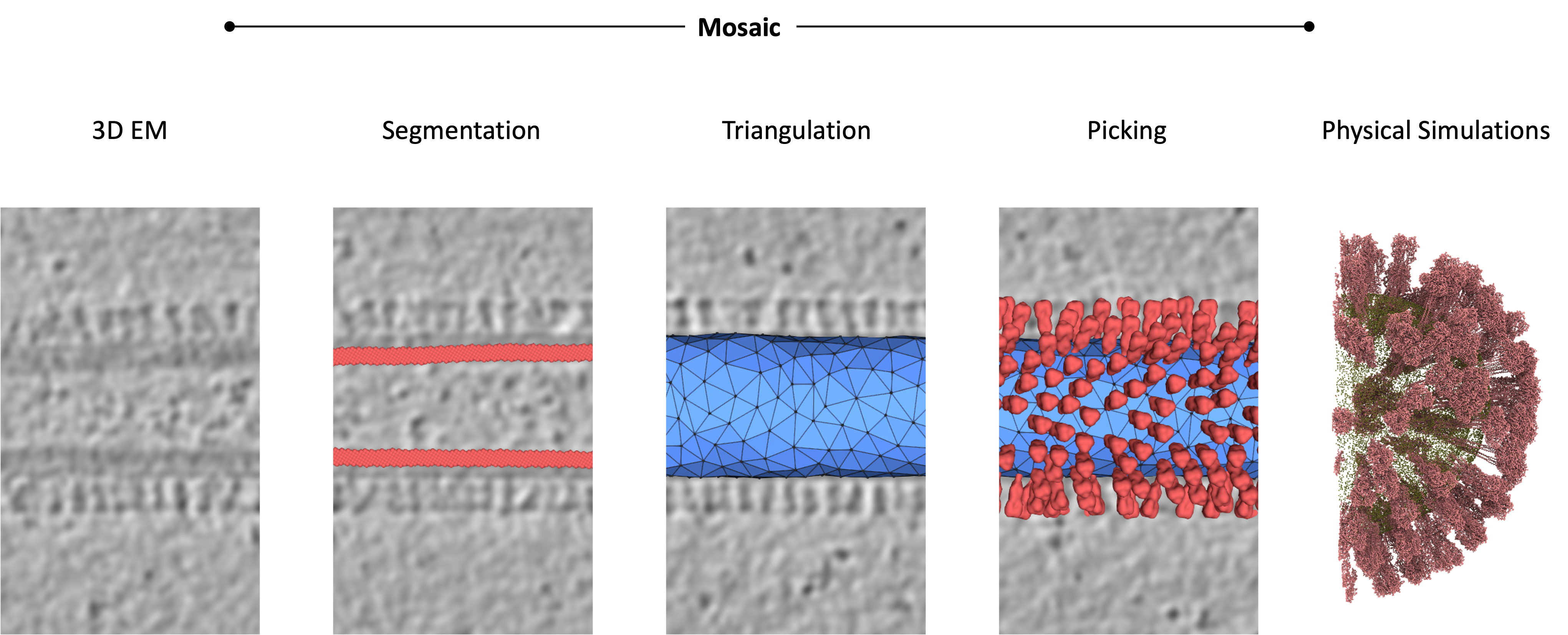
Visual Demonstration

Membrane Segmentation

1. In the Intelligence tab, click the arrow next to Membrane and configure:

   • Model: select the downloaded checkpoint file

   • Window Size: 160, Output Sampling: 12.0

   • Clustering: Enabled, Augmentation: Enabled

2. Click Apply and select the IAV VLP tomogram upon completion.

Note

Without a GPU, use the segmentation from ownCloud and load via File > Open.

Mesh Creation

Clean the Segmentation

1. In the Segmentation tab, select the Cluster section in the Object Browser

2. Click Select from Base operations and use the threshold slider to isolate the central IAV VLP

3. Close the selection window and press delete to remove small artifact clusters

4. Press r to activate the crosshair selector, then click-drag to select incorrectly segmented voxels near the tomogram edge. Press delete to remove them.

5. Select the VLP in the Object Browser:

   • In the Segmentation tab, click the arrow next to Skeletonize and choose outer_hull, click Apply

   • Select the result, click Downsample, choose Center of Mass with Radius: 48, click Apply

   Changed in version v1.1.0: Thin was renamed to Skeletonize. The outer method was replaced by outer_hull.

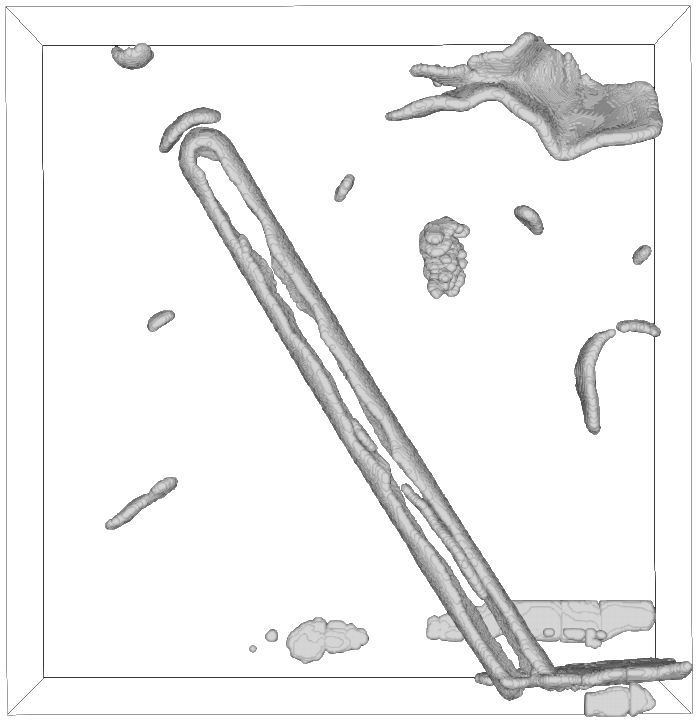
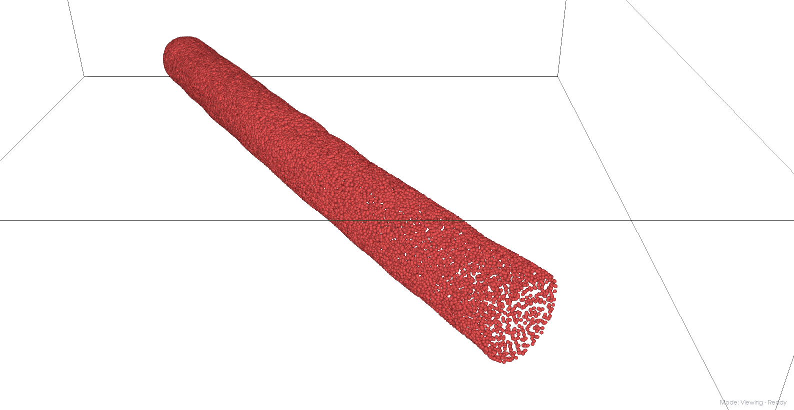
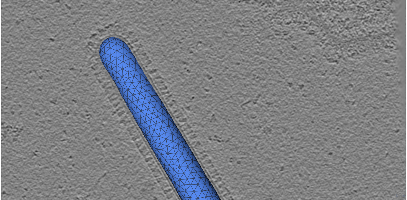
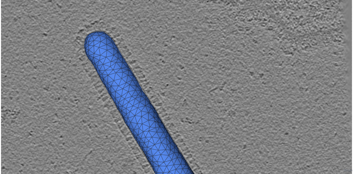
Before cleanup

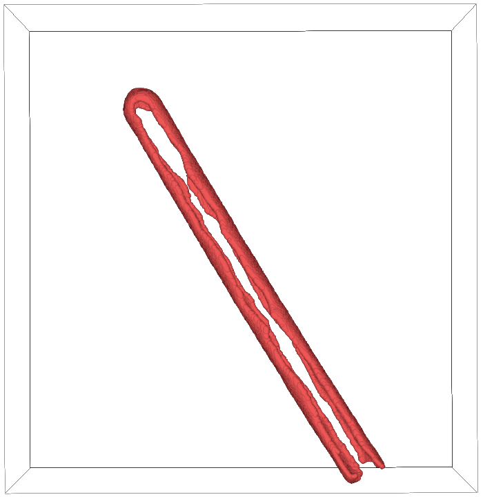
After cleanup

Generate Initial Mesh

1. In the Parametrization tab, select the cleaned segmentation

2. Click the arrow next to Mesh and configure:

   • Method: Ball Pivoting

   • Smoothness: 1.0, Curvature Weight: 1.0, Pressure: 0.0

   • Boundary Ring: 0, Radii: 60.0, Hole Size: Auto, Edge Length: 36

   Edge Length controls the resolution of the output mesh. A value of -1 (Auto) defaults to the input point spacing, in this case 48 Å from the previous downsampling step. Lowering the value produces smoother meshes at the cost of longer computation times.

   Changed in version v1.2.1: Elastic Weight renamed to Smoothness. Volume Weight renamed to Pressure. Neighbors, Downsample, and Smoothing Steps were removed. Edge Length did not exist. Sensible parameters are Elastic Weight: 1.0, Curvature Weight: 10.0

3. Click Apply. Right-click the new mesh in the Object Browser and set Representation to Mesh.

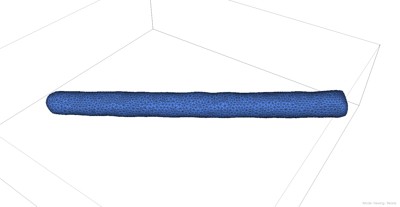
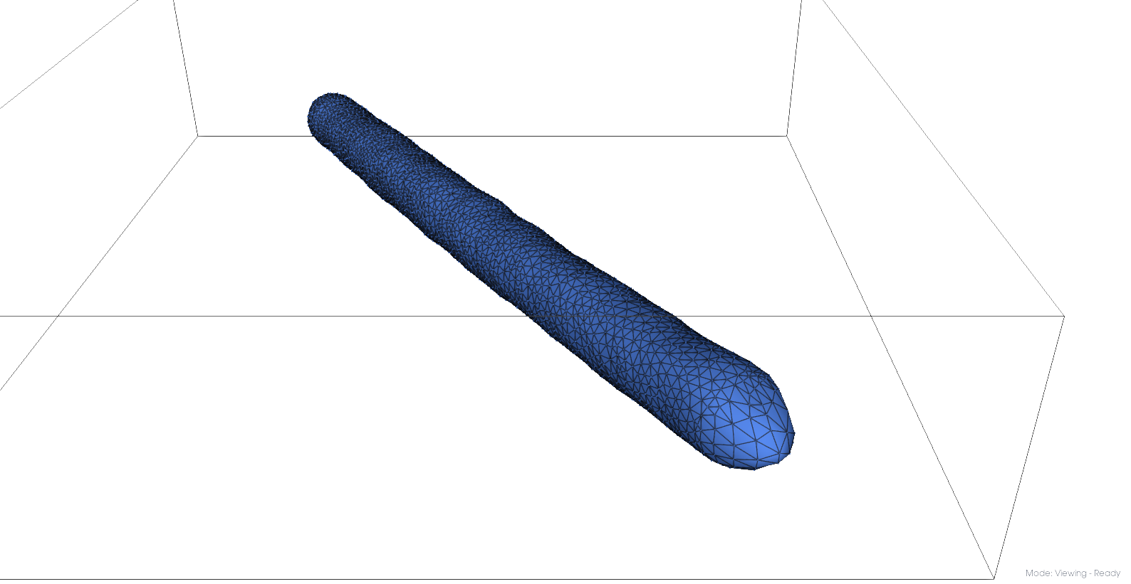
Initial mesh

Refine the Mesh

One cap of the VLP falls outside the tomogram. We resample and re-mesh to fill it:

1. Select the mesh, click Sample (Method: Points, 30000)

2. Select the sampled points, Mesh with the same settings, except Pressure 50

   Changed in version v1.2.1: Volume Weight was renamed to Pressure. Use Volume Weight: 0.005 pre 1.2.1.

The filled cap should now extend beyond the original segmentation.

Cleaned mesh points

Pressurized mesh

Equilibrate the Mesh

1. Select the refined mesh, go to Intelligence tab, click Equilibrate

2. Set Average Edge Length: 100, Steps: 5000

This produces three meshes: mesh_base (input), mesh_remeshed (target edge length), and mesh_equilibrated (equilibrated via Trimem [3]). If you want to inspect them, load the output meshes via File > Open.

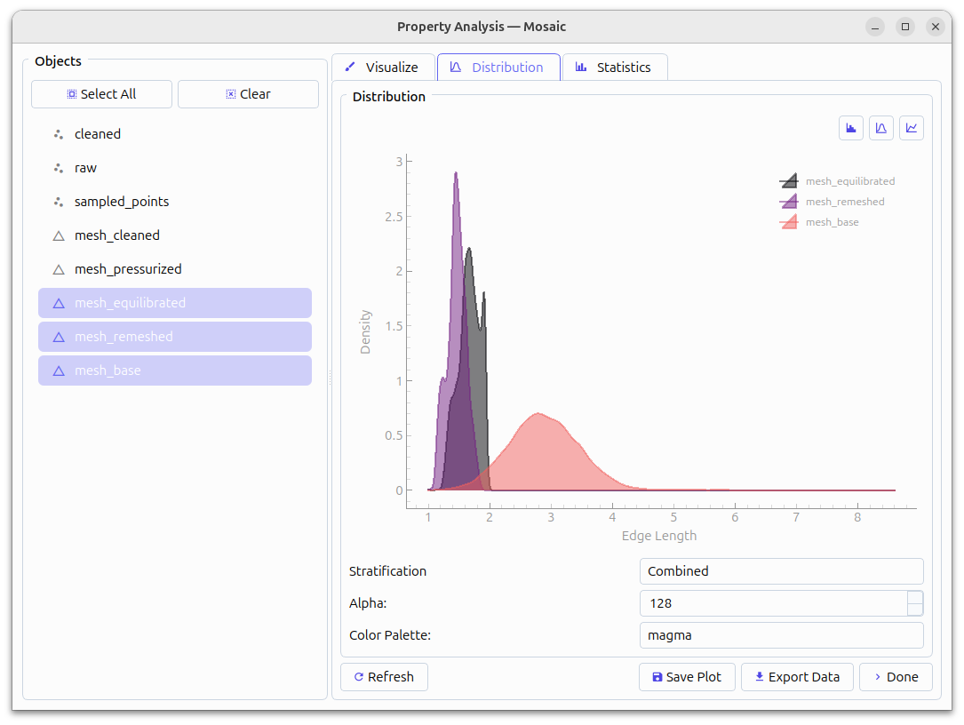
Comparison of edge lengths

An important quality metric is the edge-length distribution of equilibrated meshes. We can assess that using Segmentation > Properties, Category: Mesh, Property: Mesh Statistics, Type: Edge Length. The best initial mesh for simulation recapitulates the input geometry and has a tight edge length distribution between 1 - sqrt(3). Typically, mesh_equilibrated is the most suitable for subsequent simulation and we will use it for this example as well.

Note

Pre-computed meshes are available from ownCloud.

HMFF Simulation

HMFF simulation setup

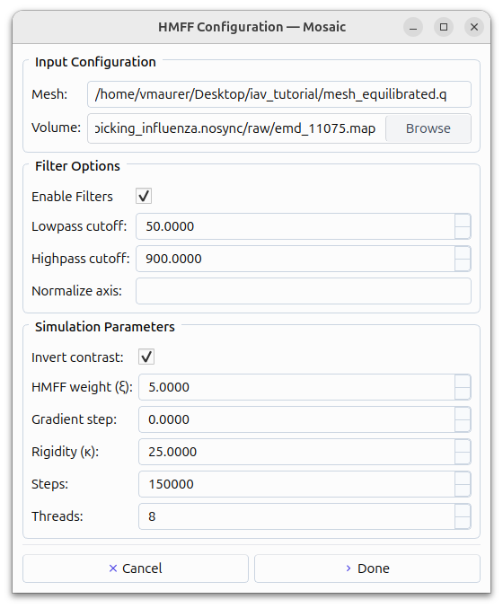
1. Go to the Intelligence tab, click DTS

2. Set parameters:

   • Mesh: mesh_equilibrated.q, Output: Up to you

   • Temperature: 1.5, Edge length: 1.0 - 4.0, Steps: 150000, Threads: 8

   • Rigidity (κ): 25.0, VolumeCoupling: SecondOrder 0.6 1000 1.1

   • HMFF weight (ξ): 5.0, Enable Filters: 50Å, Highpass: 900Å

   • Extra Parameters: AlexanderMove = MetropolisAlgorithmOpenMP 0

3. Click Setup to generate the DTS directory

The edge length parameter is related to mesh quality, and FreeDTS will inform you if any edges fall outside this range. The ideal range is 1.0 - 3.0, but upper bounds of 5.0 can still yield stable simulations. Beyond that input mesh quality should be improved. When using meshes created without the Equilibrate functionality, you need to set HMFF scale and offset parameter yourself (see mosaic.meshing.hmff equilibrate_fit for how we compute them).

After the background job has completed, navigate to your chosen output directory and from within run_1 execute:

bash run.sh

Note

Simulation outputs are available on ownCloud in hmff/TrajTSI_Done.

To load results, move to the Analyze tab within the DTS dialog, set the path to what you chose for Output in the Configure page, and load the import button in the actions field of the corresponding run.

Changed in version v1.2.4: Use the Setup dialog pre 1.2.4. The parameters remain the same, but you will have to adapt the AlexanderMove and VolumeCoupling parameters in the corresponding input.dts file manually.

Pre 1.2.4, trajectories had to be imported exclusively using the Trajectory button in the Intelligence tab using the scale parameters from the input.dts, in this case Scale: 0.012202743213335199 and Offset: 21.0,6.0,16.0. Its recommended to use the DTS dialog import, as this will include a range of properties for subsequent analysis through Segmentation > Properties > Vertex Properties.

Use View > Trajectory player to navigate time points and View > Volume Viewer to overlay the density.

Initial mesh

HMFF-refined mesh

Note

Frozen vertices indicate the simulation cannot develop them. Try increasing Min_Max_Lenghts or lowering the equilibration edge length.

Constrained Template Matching

Generate Seed Points

1. Select your desired trajectory time-point, right-click and Duplicate

2. In Parametrization, configure Sample: Method: Distance, Sampling: 40, Offset: 100

This places seed points ~40Å apart with a 100Å offset (roughly the center height of HA/NA). Export as STAR via right-click.

Template Matching

In the Intelligence tab, click Setup under Template Matching and configure PyTME [5]:

• Data: set working directory, paths to EMD-11075 and HA/NA structures

• Preprocess: Lowpass: 15, Align Template Axis: z, Flip Template: checked

• Matching: Angular Step: 7, Score: FLC, seed points STAR file, Rotational Uncertainty: 15, Translational Uncertainty: (6,6,10) for HA / (6,6,12) for NA, Tilt Range: 60,60, Wedge Axes: 2,0, Defocus: 30000, No Centering: checked

• Peak Calling: PeakCallerMaximumFilter, 10000 peaks, Min Distance: 7 (HA) / 10 (NA)

• Compute: set cores, memory, backend: cupy

Click OK to generate and run the matching scripts.

Note

Results are available from ownCloud.

Refine Protein Picks

1. Keep the top 97% of NA picks by score

2. Visualize and manually refine picks in Mosaic using the selection tool

3. Remove HA picks within 7 voxels of NA picks to resolve clashes

Filtering scripts: pytme/filter.py and pytme/resolve_clash.py on ownCloud.

Coarse-Grained Martini Models

Backmapping

1. In Intelligence, click Backmapping, select an output directory

2. Set target edge length to 20, add HA and NA inclusions

Tip

The output also contains mesh.tsi for equilibrium DTS simulations with protein inclusions.

Coarse Graining

Edit martinize.sh to add PDB paths for NA_STRUCTURE and HA_STRUCTURE, then:

bash martinize.sh

Note

Protein principal axes must align with z. An example rotation script is available on ownCloud (pytme/templates/rot_structures.py).

Create the coarse-grained system using TS2CG [6]:

bash plm.sh   # Create bilayer
bash pcg.sh   # Populate with lipids

This produces system.gro for MD simulation or visualization.

Equilibration

Gromacs [7] settings for Martini [8] equilibration are on ownCloud (ts2cg folder):

bash equilibrate.sh

Energy minimization runs on a laptop. The final equilibration step should run on an HPC cluster (see eq/equilibrate.sbatch).

References

[1]

Peukes, J., Xiong, X., Erlendsson, S., Qu, K., Wan, W., Calder, L.J., Schraidt, O., Kummer, S., Freund, S.M.V., Kräusslich, H.G., Briggs, J.A.G. (2020). “The native structure of the assembled matrix protein 1 of influenza A virus”. Nature, 587, 495-498. https://doi.org/10.1038/s41586-020-2696-8

[2]

Lamm, L., Sieber, J., Chung, J.E. et al. (2024). “MemBrain-seg: Deep learning-based segmentation of cellular membranes in cryo-electron tomography”. bioRxiv, doi.org/10.1101/2024.01.05.574336

[3]

Siggel, M., Kehl, S., Reuter, K., Köfinger, J., Hummer, G. (2022). “TriMem: A parallelized hybrid Monte Carlo software for efficient simulations of lipid membranes”. Journal of Chemical Physics, 157, 174801. https://doi.org/10.1063/5.0101118

[4]

Pezeshkian, W., Ipsen, J.H. (2024). “Mesoscale simulation of biomembranes with FreeDTS”. Nature Communications, 15, 548. https://doi.org/10.1038/s41467-024-44819-w

[5]

Maurer, V.J., Siggel, M., Kosinski, J. (2024). “PyTME (Python Template Matching Engine): A fast, flexible, and multi-purpose template matching library for cryogenic electron microscopy data”. SoftwareX, 25, 101636. https://doi.org/10.1016/j.softx.2023.101636

[6]

Pezeshkian, W., König, M., Wassenaar, T.A., Marrink, S.J. (2020). “Backmapping triangulated surfaces to coarse-grained membrane models”. Nature Communications, 11, 2296. https://doi.org/10.1038/s41467-020-16094-y

[7]

Abraham, M.J., Murtola, T., Schulz, R., Páll, S., Smith, J.C., Hess, B., Lindahl, E. (2015). “GROMACS: High performance molecular simulations through multi-level parallelism from laptops to supercomputers”. SoftwareX, 1-2, 19-25. https://doi.org/10.1016/j.softx.2015.06.001

[8]

Souza, P.C.T., Alessandri, R., Barnoud, J., Thallmair, S., Faustino, I., Grünewald, F., Patmanidis, I., Abdizadeh, H., Bruininks, B.M.H., Wassenaar, T.A., Kroon, P.C., Melcr, J., Nieto, V., Corradi, V., Khan, H.M., Domański, J., Javanainen, M., Martinez-Seara, H., Reuter, N., Best, R.B., Vattulainen, I., Monticelli, L., Periole, X., Tieleman, D.P., de Vries, A.H., Marrink, S.J. (2021). “Martini 3: a general purpose force field for coarse-grained molecular dynamics”. Nature Methods, 18, 382-388. https://doi.org/10.1038/s41592-021-01098-3