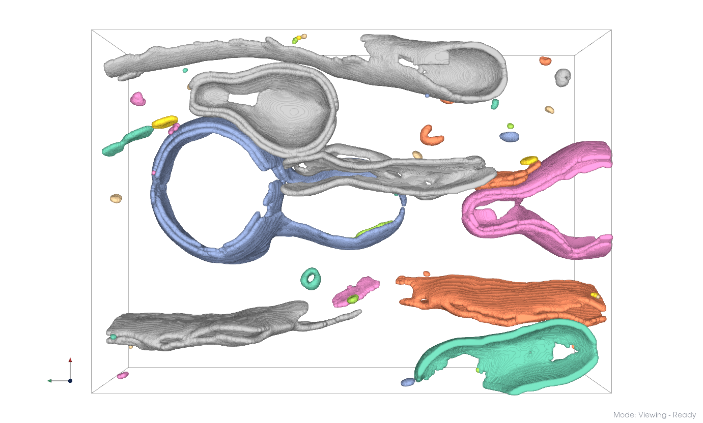
Working with in situ data#
This guide outlines strategies for analyzing in situ membrane segmentations using Mosaic, demonstrated on a Giardia lamblia dataset.
Segmentation#
Load your segmentation via File > Open or drag and drop it into the viewport. If you don’t have one, follow the membrane segmentation guide.
For large datasets, adjust the interaction point budget via the Settings button (top-right gear icon). Ultra disables interaction decimation entirely; Balanced lets you set a point budget with a slider.
Changed in version v1.3.0: Rendering presets were simplified to Ultra (no LOD) and Balanced (configurable point budget). The settings moved from Preferences > Appearance to the Settings button in the toolbar.
Raw membrane segmentation#
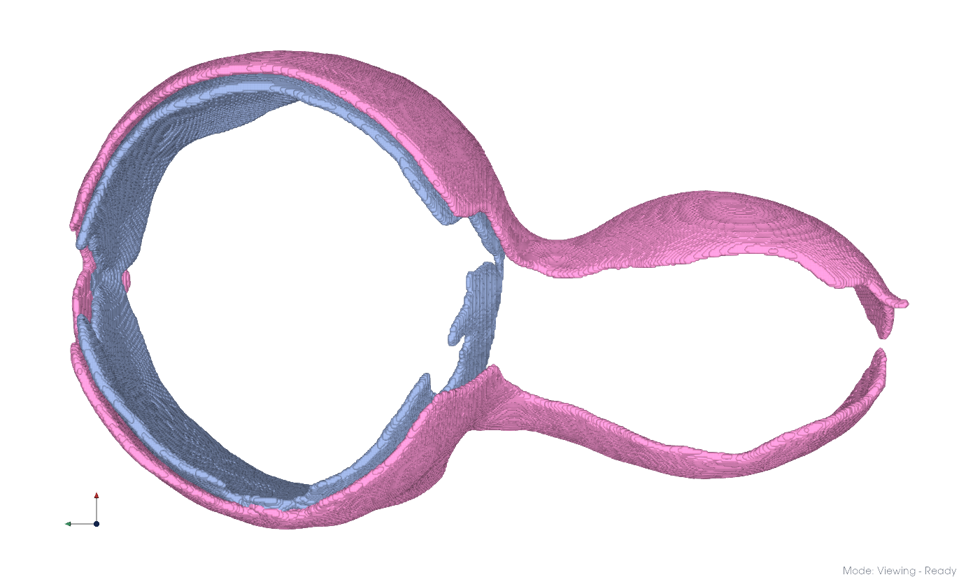
Connected Components#
Separate the dataset into disjoint membrane partitions:
Select the segmentation in the Object Browser
In the Segmentation tab, click Cluster and configure:
Method: Connected Components
Use Points: Check, Drop Noise: Check, Distance: Auto (-1.0)
You can color objects by entity using View > Coloring > By Entity.
Separated membrane components#
Tip
Distance defaults to single-voxel connectivity derived from the object’s sampling rate. Increase it to bridge gaps of multiple voxels.
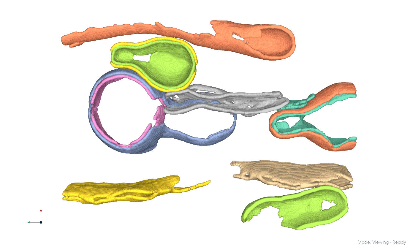
Refinement#
Remove small erroneous clusters using size-based filtering:
Click Select in the Segmentation tab
Adjust cutoffs to identify suitable size ranges (here, <25,000 voxels)
Click Remove
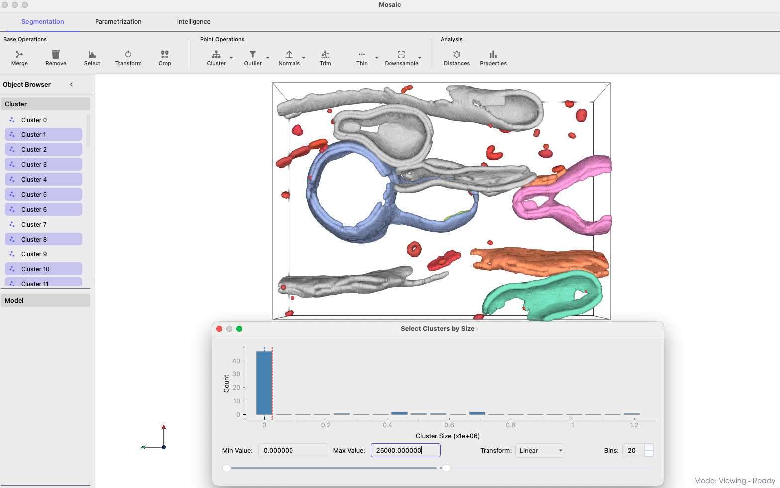
Size-based cluster filtering#
You can also interact with data directly through the viewport. Press r to activate crosshair selection for picking points or regions, and e to pick individual geometries. For lamella-style editing, use the Trim tool.
Clustering#
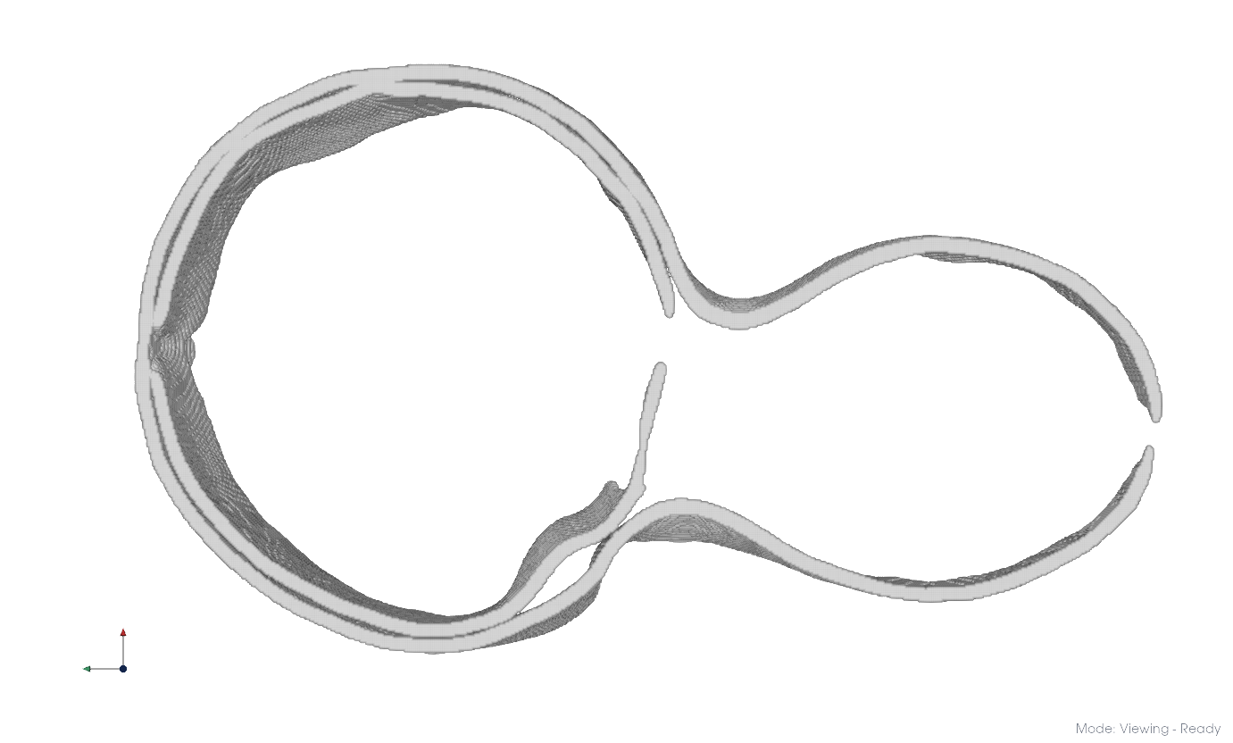
Some membrane systems (e.g. double membranes) remain merged after connected components. Graph-based clustering can separate them.
Envelope Extraction#
Optionally thin membranes to their envelope first, reducing computation and improving separation:
Select the target cluster
Click Cluster and configure:
Method: Envelope
Use Points: Check, Distance: Auto (-1.0)
Note
Check Drop Noise to add the inner membrane part as a second cluster.
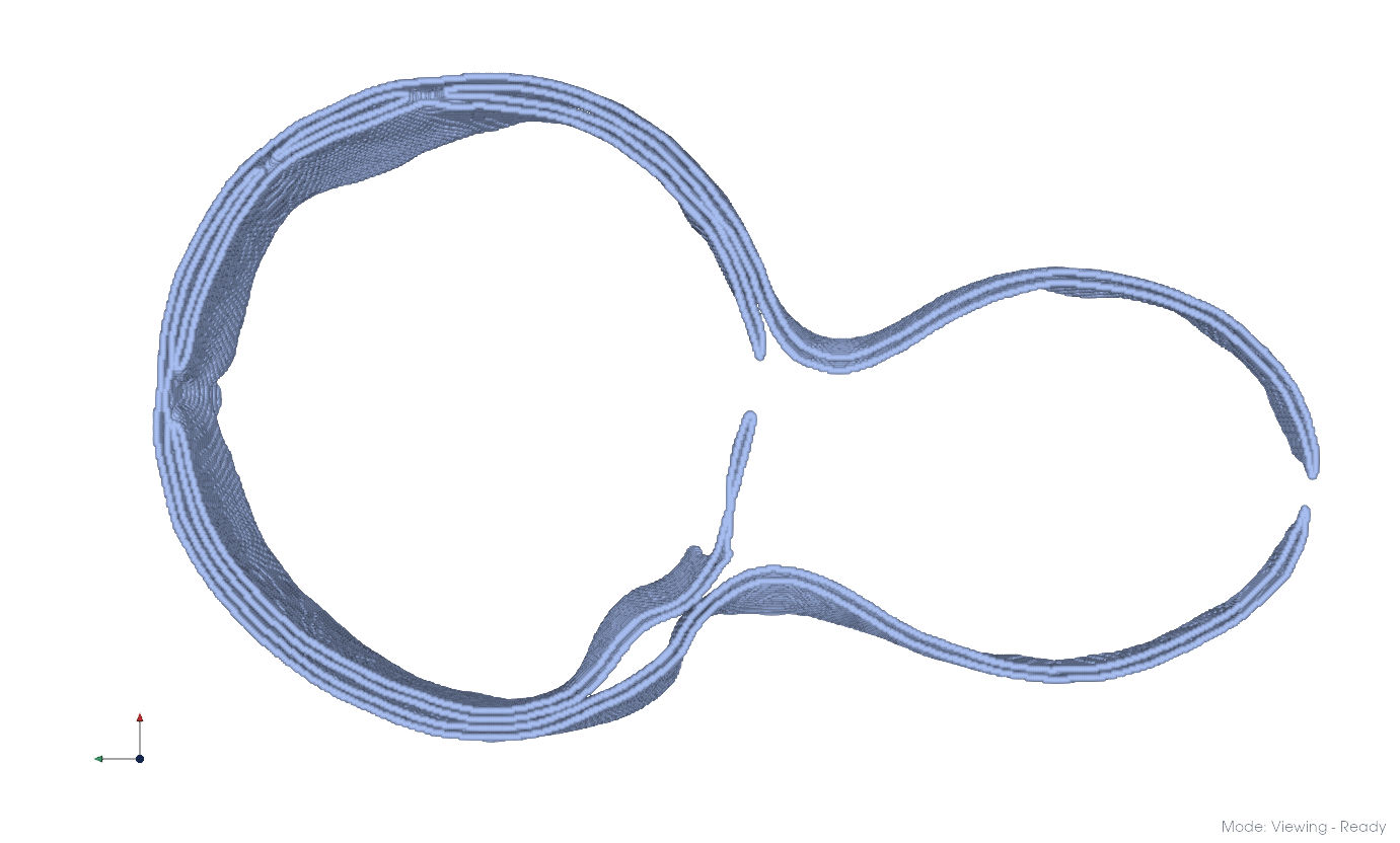
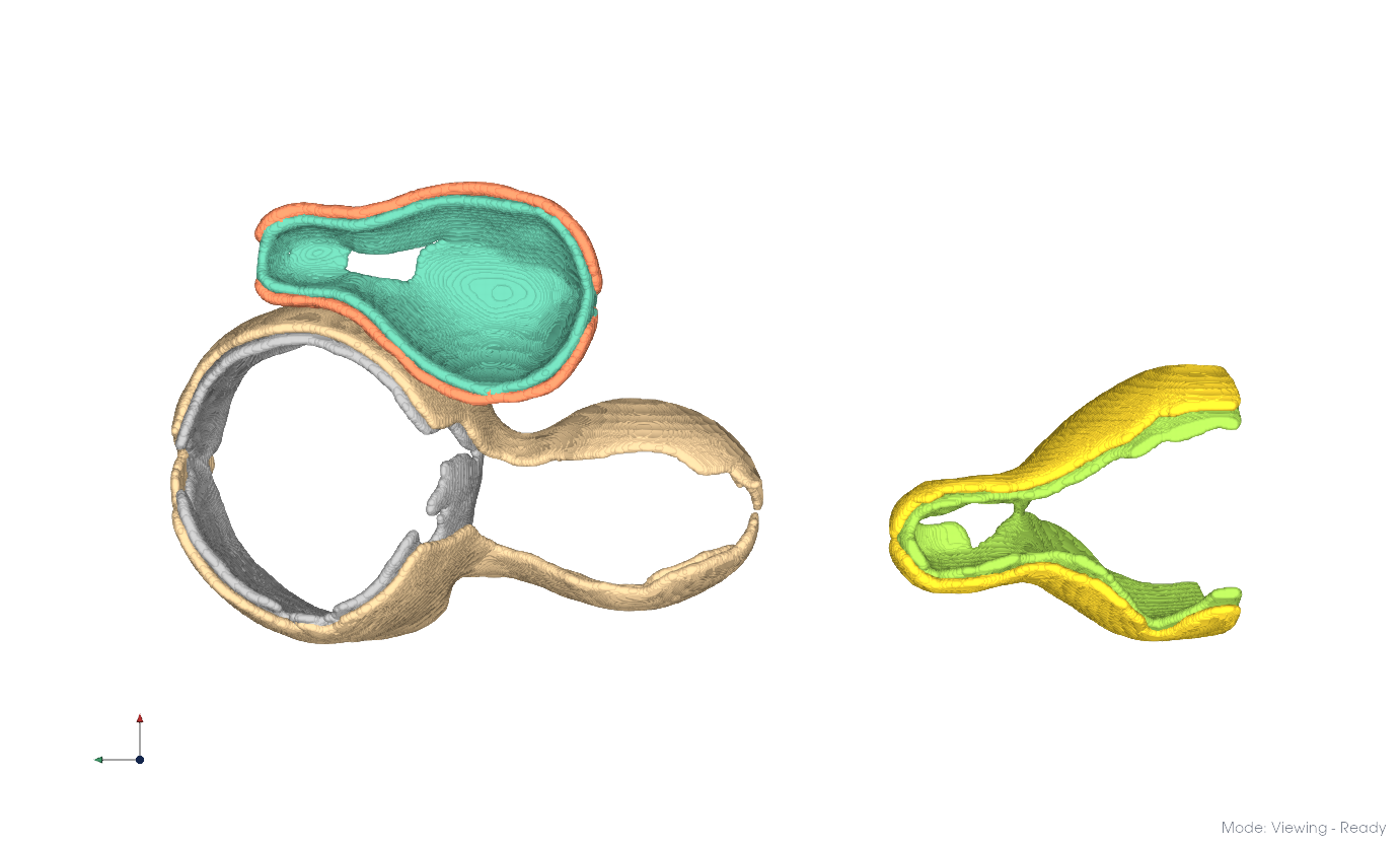
Leiden Clustering#
Leiden clustering uses graph connectivity to separate membrane systems. Whenever you have an object whose parts should be separable based on shape imposed by local connectivity, Leiden is a good choice. The resolution parameter controls fineness, start at -7.3 and increase in steps of 1.0.
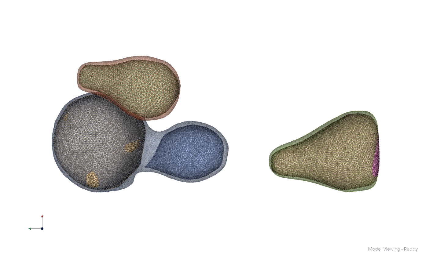
Here, resolution -7.3 yielded two clusters. Repeating at -6.3 for each produces the results below. Merge the resulting clusters into distinct membrane systems by selection.
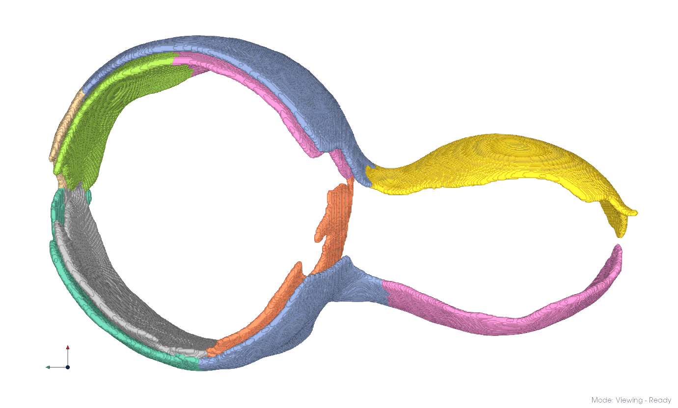
Repeat for the remainder of the dataset.
Clustering applied to the entire dataset.#
Tip
When connectivity alone is insufficient, use distance-based methods like K-Means. DBSCAN and Birch can also work but are harder to tune.
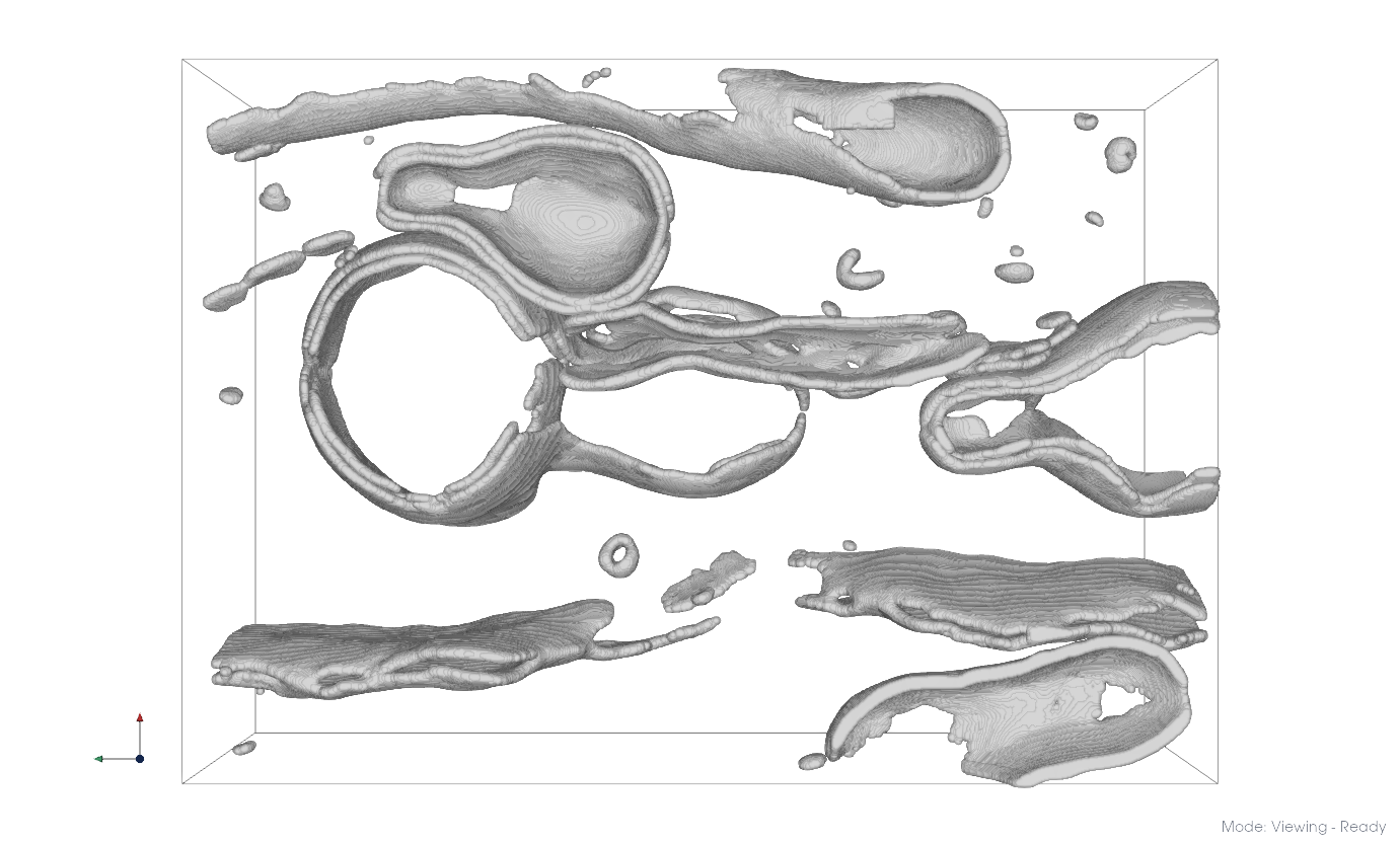
Meshing#
Meshing algorithms reconstruct a surface from a set of input points. Dense segmentations (hundreds of thousands of voxels) should almost never be meshed directly (unless you are using the Flying Edges method, which operates on voxel grids natively). The high point density doesn’t improve the mesh and makes computation unnecessarily slow. Instead, reduce the input first using for instance:
Skeletonize (Segmentation tab) to extract the structural center or boundary of the membrane, typically reducing point count by an order of magnitude while preserving shape.
Downsample > Center of Mass (Segmentation tab) to merge nearby points into centroids at a controllable radius, producing uniform spacing without changing the geometry’s extent.
Either produces a lightweight point cloud that meshes quickly and cleanly.
Fit triangular meshes to the reduced point clouds:
Select membrane clusters in the Object Browser
In the Parametrization tab, click Mesh and configure:
Method: Alpha Shape
Smoothness: 1.0, Curvature Weight: 1.0, Pressure: 0.0
Boundary Ring: 1, Alpha: 1.0
Changed in version v1.2.1: Elastic Weight renamed to Smoothness (rescaled). Volume Weight renamed to Pressure. Neighbors, Scaling Factor, and Distance were removed. Curvature Weight: 10.0 is sensible pre 1.2.1.
Alpha shapes work well for convex membrane morphologies. For non-convex membranes, use Ball Pivoting (e.g. with core-thinning via Skeletonize at radius 40, then Ball Pivoting at radius 50). Poisson reconstruction also produces complete meshes using a different completion strategy.
Changed in version v1.1.0: Thin was renamed to Skeletonize.
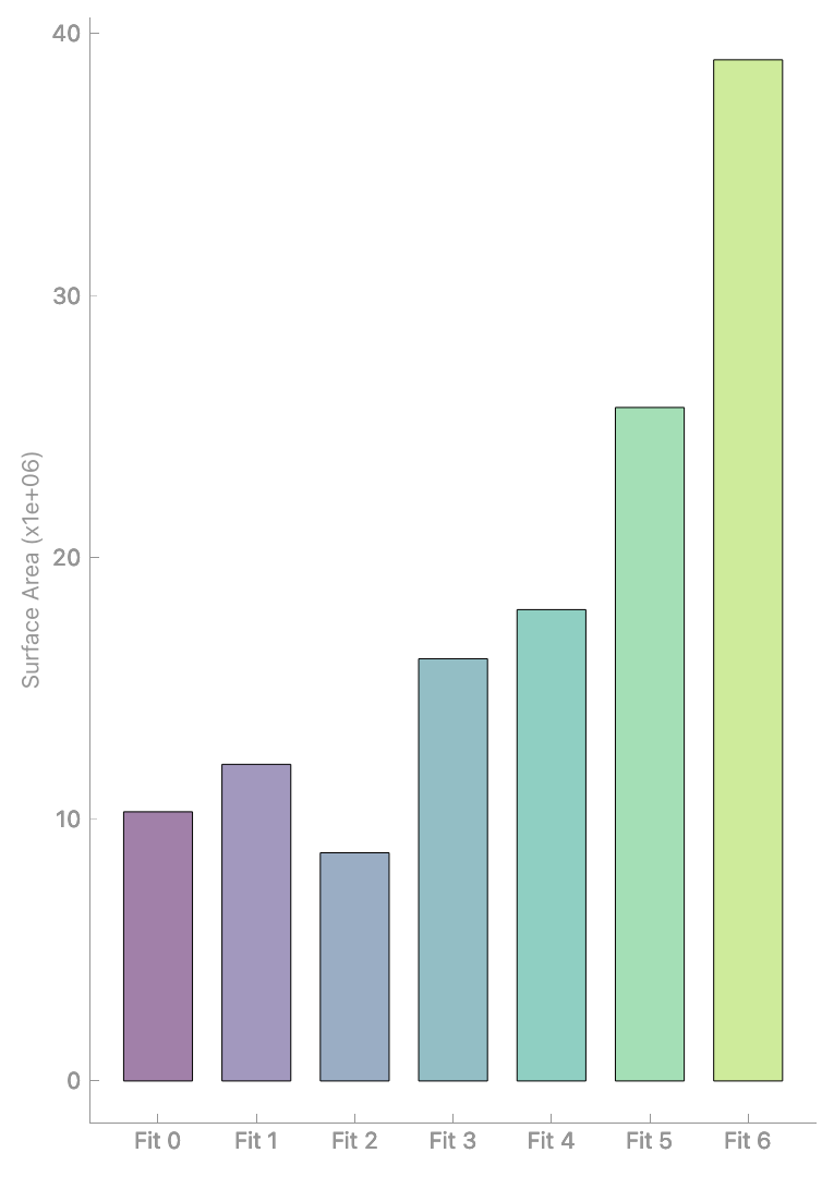
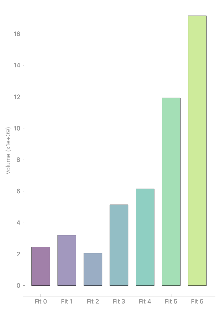
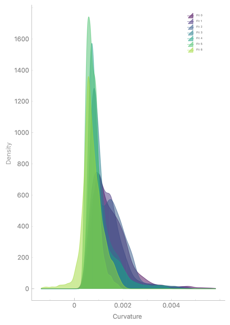
Analyze geometric properties via Segmentation > Properties:
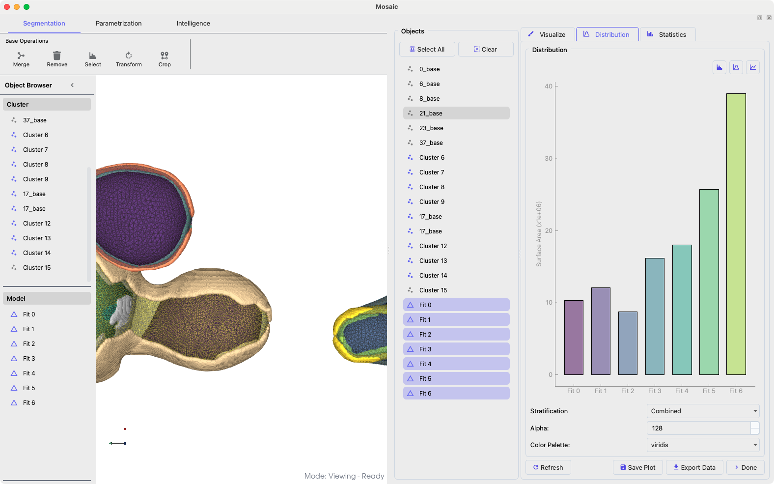
Analyzing mesh properties.#